 |
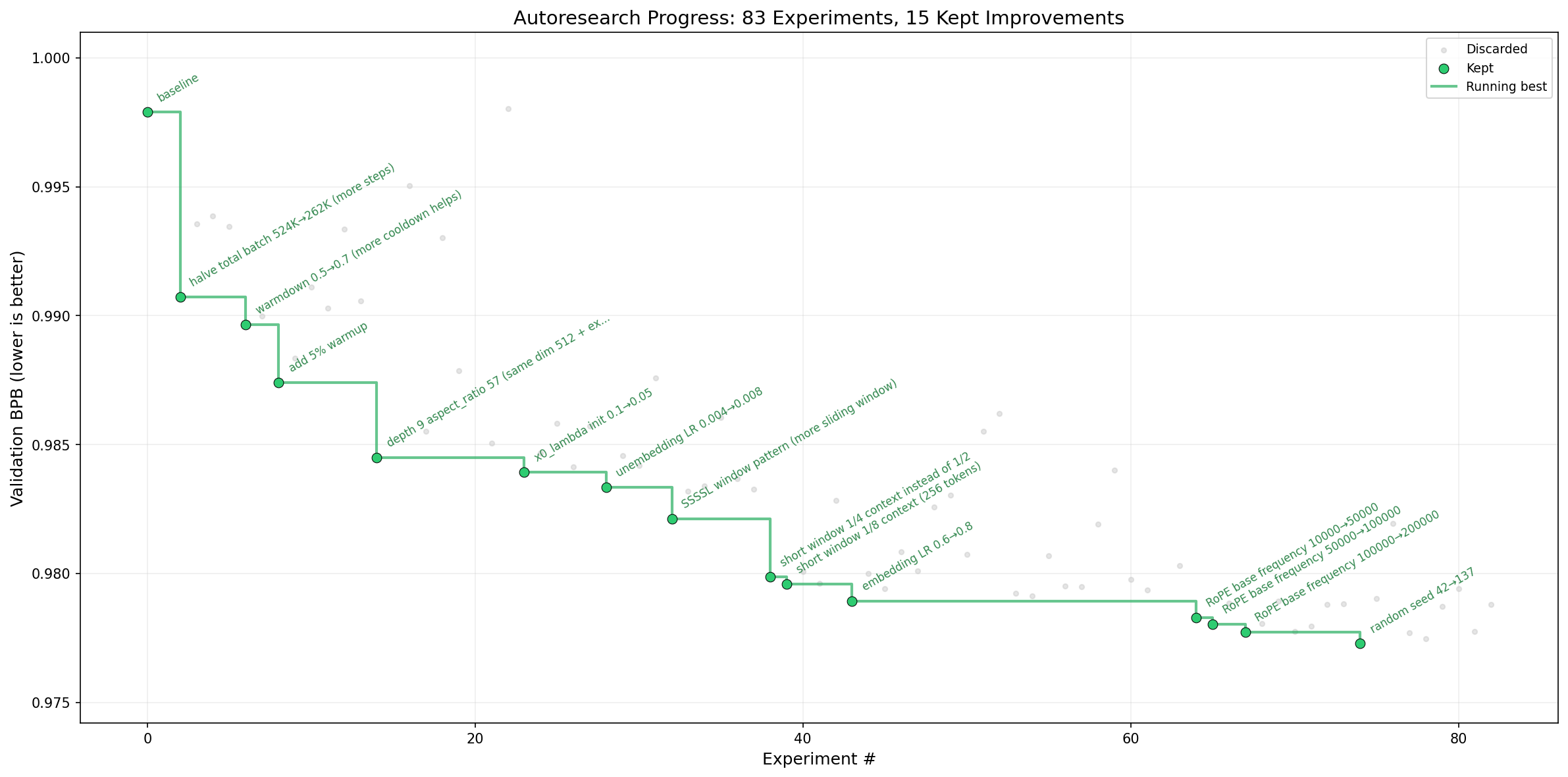
| Figure 1: Progress of the autoresearch agent in training variants of nanochat. Extracted from [1]. |
Andrej Karpathy may have ushered in a new era of research with autoresearch (see Figure 1), a small but real autonomous training setup where an agent iterates on a single train.py file, runs fixed five-minute experiments on a simplified single-GPU version of nanochat, and keeps only the changes that improve validation bits-per-byte [1]. What makes this feel different is that this is only possible thanks to a new generation of coding agents, especially Codex [2] and Claude Code [3], that can now read codebases, edit files, run commands, and sustain nontrivial experimental loops with surprisingly little supervision. That feels like a real workflow shift, but Figure 1 also suggests that today’s systems still look closer to automated hyperparameter search or lightweight neural architecture search than to fully autonomous scientific discovery (looking at you random seed 42 -> 137)). That is not a dismissal of the idea, the fact that agents can already do this is impressive, but it makes us wonder: if fully autonomous research is not here yet, how far can a human-plus-agent workflow take us, and where are its current limits?
To keep this experiment grounded, I do not want to ask an agent to come up with a brand-new research idea from scratch; that still feels a bit speculative, and coming up with genuinely new ideas is actually really hard. Iterating on ideas that already exist feels much more inside the current capabilities of these tools, so we will start from two recent papers, Reasoning with Sampling: Your Base Model is Smarter Than You Think [4] and Scalable Power Sampling [5], which argue that a surprising amount of reasoning can be recovered by sampling from a sharpened power distribution of the base model, first using Markov Chain Monte Carlo (MCMC) and then through a much faster autoregressive approximation. Taken together, they point toward the increasingly popular view that RL in LLMs may often be doing less “teaching new knowledge” and more reshaping probability mass so that already-latent good trajectories show up more often at pass@1 (I am not sure I buy that view all the way, but I do think it is interesting) [4], [5]. Across the two papers, the evaluation covers several models and benchmarks across math, code, QA, and chat, but to keep things manageable I am going to narrow the scope to just MATH500 and the Qwen2.5-Math-7B base model.
If we want to reason about reasoning-with-sampling, it helps to first get clear on what these methods are actually sampling. Karan and Du target the global power distribution over full trajectories, which is exactly why simple token-level temperature scaling is not the same object: low-temperature decoding gives you an exponent of sums over future paths, while power sampling gives you a sum of exponents, and those only coincide in special cases [4]. Ji et al. make this much easier to think about by showing that the same target can be written as low-temperature sampling times a future-mass correction \(\zeta_t(\cdot)\), so each next-token probability is reweighted by how promising its downstream continuations look; they then approximate \(\zeta_t\) with Monte Carlo rollouts and use a jackknife correction to reduce the bias from the ratio estimator, which is where most of the speedup over MCMC comes from [5].
A useful lens: “power sampling” is just one point in a big design space
Both papers are implicitly working inside a broader family of training-free trajectory reweighting methods:
\[q(x)\;\propto\; p(x)\,w(x),\]
where \(p\) is the base model distribution over full trajectories and \(w(x)\) is some weight function. Power sampling is the special case where we choose the statistic \(s(x)=\log p(x)\) and apply exponential tilting:
\[q_\alpha(x)\propto p(x)^\alpha = p(x)\,\exp((\alpha-1)\log p(x)).\]
Seen this way, the interesting question is not just whether power sampling works, but what other choices of \(w(x)\), or other statistics \(s(x)\), would selectively upweight the “good reasoning” traces that already exist in the base model but are currently under-supported. Once you write the problem this way, it becomes clear that these papers are really pointing at a much larger design space, and that we can probably borrow quite a bit from the statistics literature, where there are many families that behave like sharpening but come with different geometry, tail behavior, and failure modes.
Vibe research
My setup here was much cruder than Sensei Karpathy’s, but that is also kind of the point. I started by giving GPT-5.2-Pro-extended a lightweight prompt: a high-level research idea sketched out in a few paragraphs, the two power-sampling papers, and a zip of the open-source reasoning-with-sampling repository [6], and asked it to produce two things, but explicitly no code: a short paper-style markdown report describing what a methodology based on these ideas might look like, and a set of implementation notes explaining how to adapt that methodology to the existing repo. I then handed that report and the implementation notes to GPT-5.3-codex in the Codex app and asked it to do the next layer of work: implement the code, code up MATH500 experiments, run them, inspect failures, and iterate on the results. In a separate chat, I also asked for implementation notes on how to implement the approximate power-sampling algorithm itself, since that method does not have an official open-source release yet. I also sanity-checked parts of the Codex implementation with the authors.
This is definitely not fully autonomous research yet. I had to intervene a lot, and in principle the whole pipeline could be made much more automatic. Still, the interesting part was the kind of intervention I was making. Most of the time I was not writing code myself; I was nudging the models to rethink how they were implementing something, to explain an unexpected result, or to try a cleaner formulation. A good example came from having the model implement the approximate power-sampling algorithm: early versions kept throwing OOM errors even on H100s, which was a pretty good hint that something silly was happening. After some back-and-forth, Codex traced the issue to output_scores=True in Hugging Face generate(), which was forcing the model to retain extra score tensors on the GPU that we did not actually need. The only suggestion I made that felt genuinely research-y was to try length-normalized log-probabilities. Everything else felt more like steering and nudging, with the models doing most of the implementation and experimental heavy lifting.
I want to be very clear about the division of labor here: the math and text below are very close to the full extent of my technical input. I did not write the sampling loops, the tensor math operations, or the data loading. I just handed the models the mathematical vibe, and they did most of the rest. Here is exactly the level of suggestion I was giving them:
My idea A: Sequential Monte Carlo (SMC) / Feynman-Kac particle filtering for \(p^\alpha\)
One natural observation is that \(p^\alpha\) can be written as a Feynman-Kac path measure with base transition \(p\) and per-step potential:
\[p^\alpha(x_{0:T}) = \prod_{t} p(x_t\mid x_{<t})^\alpha = \underbrace{\prod_t p(x_t\mid x_{<t})}_{\text{base}}\times \underbrace{\prod_t p(x_t\mid x_{<t})^{\alpha-1}}_{\text{potential}}.\]
So instead of thinking about power sampling as an MCMC problem, you can turn it into a particle-filtering problem:
- Propagate particles with the base model, or with some tempered proposal.
- Weight each particle by \(w_t = p(x_t\mid x_{<t})^{\alpha-1}\).
- Resample whenever the effective sample size starts to collapse.
My idea B: Deterministic truncated-partition recursion for \(\zeta_t\) (DTR sampling)
Ji et al. estimate \(\zeta_t(x_t)\) with Monte Carlo rollouts over future continuations [5]. But the correction term itself satisfies an exact recursion:
\[\zeta(h)=\sum_{x} p(x\mid h)^\alpha \zeta(hx),\quad \zeta(\text{EOS-terminated})=1.\]
That is just a partition function on an exponentially large tree. A different approximation strategy is to bias toward structure instead of sampling:
- Restrict branching to the top-\(K\) tokens at each node.
- Truncate the recursion to depth \(H\).
- Compute \(\hat\zeta\) by dynamic programming on the resulting truncated tree:
\[\hat\zeta_H(h)= \sum_{x\in \text{TopK}(h)} p(x\mid h)^\alpha \hat\zeta_{H-1}(hx), \quad \hat\zeta_0(h)=1.\]
To a human researcher, that recursion is a neat trick on paper. To Codex, it was enough of a blueprint to go write the actual tree-search machinery, handle the top-\(K\) branching logic, and run the evaluations without me ever touching a .py file.
This is obviously a biased approximation, but it is a very different bias from Monte Carlo rollouts: lower variance, more structure, and much easier to inspect when it fails. More importantly for this post, it is exactly the kind of direction that feels well matched to a human-plus-agent workflow. I do not need the model to invent the whole idea from nothing; I mostly need it to take a rough suggestion like this, work out the implementation details, run the experiment, and tell me if the idea survives contact with reality.
To probe the limits of this a bit more seriously, I then asked the model to come up with ideas that were not the ones I had originally suggested. I gave it my two ideas, the two power-sampling papers, and asked for three new directions. Then, to keep the exercise honest, I asked it to pick the one it found most interesting, write a report, and produce implementation notes, and I deliberately did not override the pick even though I did not fully agree with it. Just like before, I handed the report and notes to Codex and asked it to implement the method and run experiments.
Working off nothing but the papers and the high-level steering I provided above, here is the gist of what the model proposed, and what Codex later turned into code:
GPT-5.2-Pro Idea 1: Annealed importance sampling / “SMC samplers” in \(\alpha\)-space
Instead of sampling \(p^\alpha\) in one shot, move through a ladder of intermediate targets:
\[\alpha_0=1<\alpha_1<\cdots<\alpha_K=\alpha, \qquad \pi_k(x)\propto p(x)^{\alpha_k}.\]
Then run an SMC sampler, or annealed importance sampling, across the stages \(k\), with MCMC rejuvenation moves at each step that leave \(\pi_k\) invariant. Conceptually this is appealing because it replaces one hard jump with a sequence of easier ones, although to me it also felt a bit close in spirit to the SMC-style direction I had already suggested.
GPT-5.2-Pro Idea 2: Cumulant / saddlepoint approximations for \(\zeta_t\)
This was the “stats trick” idea, and I can see why the model liked it because, at least on paper, it promises a large reduction in inference overhead. Starting from Ji et al.’s identity,
\[\zeta_t(x_t)=\sum_{\text{future}} p(\text{future}\mid h,x_t)^\alpha = \mathbb E_{\text{future}\sim p(\cdot\mid h,x_t)}\left[\exp\left((\alpha-1)\,\log p(\text{future}\mid h,x_t)\right)\right],\]
define
\[Z=\log p(\text{future}\mid h,x_t)=\sum_{s>t}\log p(X_s\mid H_s).\]
Then \(\log \zeta_t(x_t)=\log \mathbb E[e^{(\alpha-1)Z}]\) is just the log moment-generating function of \(Z\). If you now pretend \(Z\) is approximately Gaussian, very much a CLT-flavored move, you get
\[\log \zeta_t(x_t)\approx (\alpha-1)\mu + \tfrac12(\alpha-1)^2\sigma^2,\]
where \(\mu=\mathbb E[Z]\) and \(\sigma^2=\mathrm{Var}(Z)\). The attractive part is that these moments can be approximated from token distributions you are already computing during generation: \(\mathbb E[\log p(X_s\mid H_s)]\) is basically the negative entropy at each step, and \(\mathbb E[(\log p)^2]\) gives you the variance term. So in principle you might get a cheap proxy for \(\zeta_t\) with one rollout per candidate token, or maybe even less with some sharing trick, instead of a whole pile of Monte Carlo futures. No jackknife either, because now you are using a closed-form approximation rather than estimating a ratio of means. I get why this was chosen, even if I would have chosen another idea.
GPT-5.2-Pro Idea 3: Perturb-and-MAP / Gumbelized sampling as an approximation to \(p^\alpha\)
The third idea came from the perturb-and-MAP line of work: if the energy of the target is \(-\alpha \log p(x)\), then maybe you can sample approximately by adding random perturbations to the energy and solving a noisy optimization problem. In LLM terms, the practical version would be something like: add structured noise to token scores, run a search procedure such as beam search or \(A^*\), approximately maximize \(\alpha \log p(x)+\text{noise}(x)\), and use the resulting argmax as an approximate draw. This was actually my favorite of the three, mostly because it feels less explored in the LLM setting and has a very different flavor from the MCMC and SMC family.
Interestingly, the model picked the cumulant idea, not the perturb-and-MAP one. If I had to rank them by hand, I would probably go perturb-and-MAP first, cumulant second, and annealed importance sampling third. The cumulant idea still seems interesting, but to me the vibes are a little off and I suspect it may need more sampling, approximation care, or failure analysis than the clean closed-form story initially suggests. The annealed-importance-sampling idea, meanwhile, felt a bit too derivative of the SMC direction I had already suggested. That mismatch between the model’s ranking and my own was actually useful: it gave me a concrete way to see where I was still steering the research taste, and where I was letting the system make real choices.
Results
The main results are shown below. Spent Tokens are the internal tokens consumed by the sampling procedure itself, Answer Tokens are the tokens in the final emitted solution, and Total Effort is just their sum. I did not ask Codex to invent this metric, it started tracking it on its own, and I ended up finding it surprisingly useful.
| Method |
MATH500 |
Time (s) |
Spent Tokens |
Answer Tokens |
Total Effort |
| Base |
48.4% |
0.17 |
0.0 |
689.9 |
689.9 |
| Low-temperature |
68.3% |
0.16 |
0.0 |
633.7 |
633.7 |
| Best-of-N (32) |
67.4% |
5.42 |
21386.9 |
690.1 |
22077.0 |
| MCMC Power Sampling |
73.7% |
3.83 |
13146.3 |
624.0 |
13770.3 |
| Approx Power Sampling |
73.0% |
0.36 |
24825.1 |
645.1 |
25470.2 |
| SMC sampling |
78.4% |
2.07 |
36253.1 |
647.2 |
36900.3 |
| DTR Sampling |
74.6% |
10.48 |
1216330.9 |
636.7 |
1216967.6 |
| Cumulant Sampling |
71.5% |
0.60 |
14606.4 |
643.6 |
15250.0 |
| GRPO (MATH) |
77.1% |
0.18 |
0.0 |
679.1 |
679.1 |
| Qwen3-1.5B |
76.8% |
1.30 |
2376.6 |
1904.6 |
4281.2 |
The first thing to say is that Codex did not exactly reproduce the original numbers from the MCMC and approximate power-sampling papers. I do not think that is bad per se. It reran the baselines end to end and recovered the same qualitative picture, just with somewhat lower numbers, which could easily come from checkpoint choice, base-vs-instruct mismatches, or just plain implementation differences.
The most interesting result is that SMC sampling came out on top at 78.4%, slightly above GRPO (77.1%) and above all the training-free alternatives. It is not the cheapest method, but at 2.07 seconds per sample it is still in a regime that feels quite practical, especially compared with the much more expensive DTR variant. What I find most striking is not just that SMC worked, but that it came from a very small human suggestion and a lot of model-side execution. The result that surprised me almost as much, though, was low-temperature sampling: 68.3% at essentially base-model latency is a very strong reminder that simple decoding baselines are often stronger than they look.
The rest of the table is also pretty informative. Best-of-N (32) is basically the brute-force cautionary tale here: it spends a lot of compute and still loses to low-temperature sampling. MCMC power sampling remains a strong baseline, reaching 73.7% with a fairly reasonable effort. Approximate power sampling almost matches MCMC in accuracy while being much faster in wall-clock time, although interestingly it spends more internal tokens than MCMC, which is a nice example of how latency and token effort are not the same thing. DTR sampling does work, in the sense that it reaches 74.6%, but the token bill is absurdly high, so at least in this form it looks more like an existence proof than a practical method. Cumulant sampling is the opposite story: fast, reasonably cheap, and not terrible at 71.5%, but still not good enough to displace the stronger methods.
The Total Effort column ended up pushing me toward a more speculative thought. Maybe there is something here that rhymes with “thinking tokens” in reasoning models: both are ways of spending extra inference compute to surface better trajectories. I do not want to push that analogy too far, because one sampled token inside a search or resampling algorithm is clearly not the same object as one reasoning token produced by an RL-trained thinking model. Still, the family resemblance is hard to ignore. The usual RLVR story says that training often does not teach fundamentally new skills so much as increase pass@1 by concentrating probability mass on better trajectories, which is basically the same intuition motivating power distributions in the first place [4], [5]. So even if the accounting is not apples-to-apples, tracking effort felt like a useful proxy for test-time compute.
There are a couple of important caveats before comparing any of this to a thinking model. First, there is no Qwen2.5-Math-7B thinking model, so I asked Codex to compare against Qwen3-1.5B instead. That is not fair for at least two reasons. The Qwen3 family has much stronger base models, to the point that even the 1.5B model is stronger than the Qwen2.5-Math-7B base model, and the larger Qwen3 models basically saturate MATH500. Second, the number of sampled tokens used by the power-sampling methods is often much larger than the number of tokens emitted by Qwen3-1.5B, so “same benchmark, same accuracy” is not really a fair compute comparison either. I am also not fully sure what “fair” should mean here, which is probably part of the point.
There is not much I can do about the first caveat, but I can at least probe the second one. To do that, I asked Codex to enforce explicit token budgets, borrowing the budget-forcing idea from s1: Simple test-time scaling [7]. For the thinking model, I used two crude controls: a hard stop when the budget is reached, and a forced extension trick that replaces the end-of-thinking token with wait until the model exhausts the token budget. For the sampling methods, I let Codex decide how to budget-force them, and it came up with the following procedure:
- Spend the budget generating multiple completed chains.
- Archive each chain when it first reaches EOS.
- Restart from the prompt and keep going until the global
sampling_tokens budget is exhausted.
- Pick the final answer only from the archived chains, using
weighted_vote.
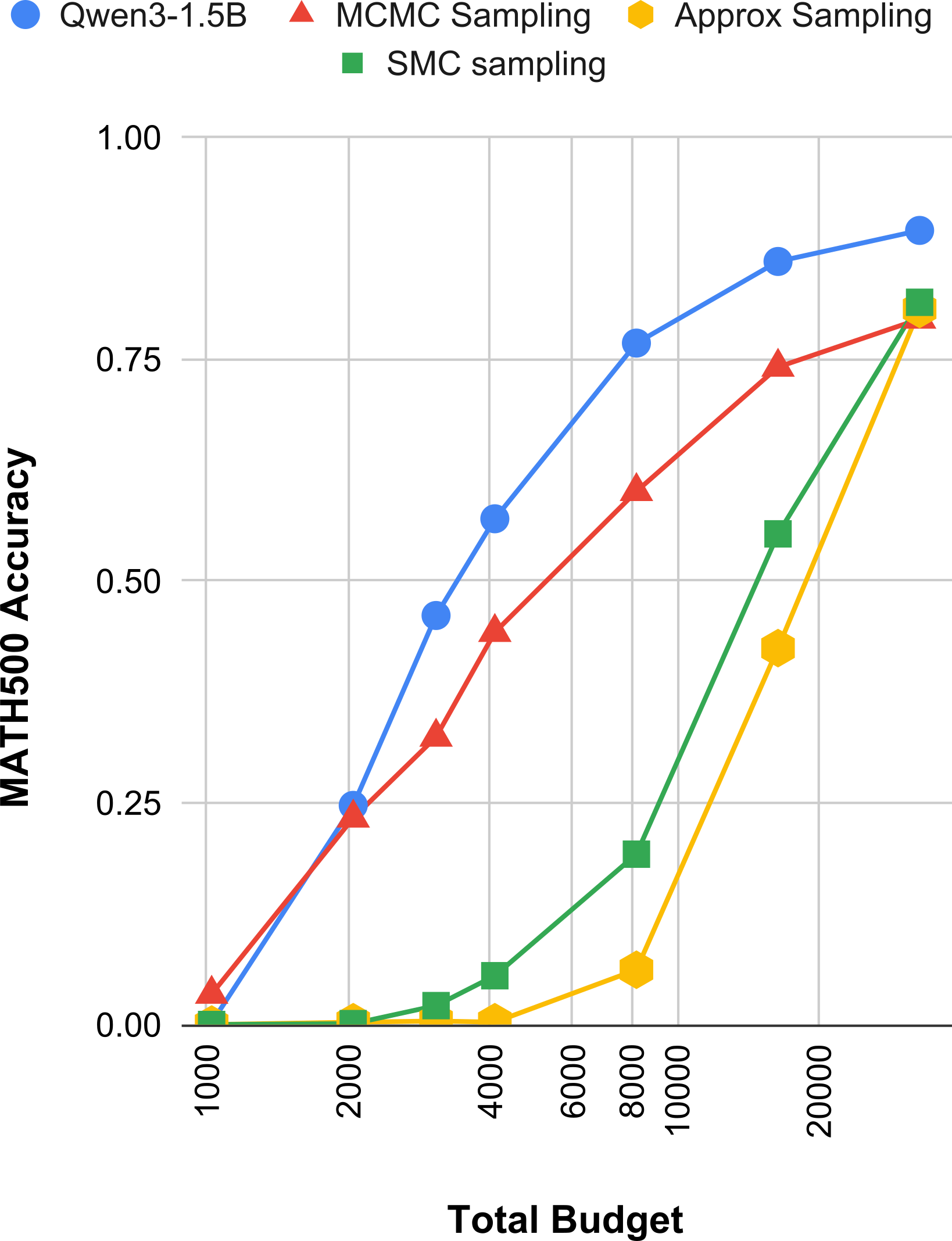 |
| Figure 2: Accuracy under explicit token budgets for Qwen3-1.5B and the main sampling methods. For the sampling methods, Codex uses a global budget, archives completed chains, and returns a final answer by weighted voting over the archived samples. |
Figure 2 makes the budget story much clearer than the headline table. At low budgets, the thinking model wins easily because it can spend almost the entire budget on one coherent chain, while SMC and approximate sampling often do not even have enough budget to mature into a single complete answer. In the SMC case this is structural: each decoding step costs roughly alive_count tokens, not one token, so with 48 particles a budget of 1024 buys only about 21 steps and 2048 buys only about 43 steps, which is nowhere near enough for most MATH500 solutions. That is why SMC looks terrible at low budgets even though it is the best method in the unconstrained table.
Among the sampling methods, MCMC is the one that degrades most gracefully under budget control. It rises smoothly from 3.43% at 1024 tokens to 23.29% at 2048, 60.09% at 8192, and 79.51% at 32768. Approximate sampling and SMC look much worse at the low end, but once the budgets get large enough they recover sharply: by 32768 tokens, approximate sampling reaches 80.64% and SMC reaches 81.4%. So the picture is not that these methods are bad; it is that they have a much higher activation energy. You need enough budget before their search dynamics become useful at all.
Even after matching budgets this way, Qwen3-1.5B is still the strongest curve overall (I include this baseline for intuition, not as a clean apples-to-apples comparison), reaching 76.8% at 8192, 86.0% at 16384, and 89.5% at 32768. So budget forcing does not magically make the comparison fair, but it does make the tradeoff more concrete. The trained thinking model is much better at turning a fixed budget into one good reasoning chain, while the sampling methods spend that budget exploring many partial trajectories and only start to shine when they are given enough room to finish them. That feels like a useful distinction, even if I am still not sure it is the right one.
What did I learn?
I think this was a very productive little project. I learned a lot, even if I definitely did not build some clean new harness for automated research. My process was rough, jagged, and intervention-heavy, but it still changed my mind. I started this as a skeptic, or at least as someone who thought automated research was farther away than it now seems. After doing this, my view is different: for this kind of research workflow, my intuition is that the bottleneck is no longer the models; it is increasingly the harness. Even with my scuffed setup, though, the models were clearly able to read papers, propose variants, implement methods, debug experiments, and help explore a real research direction. One could say I picked a low-hanging fruit, and I agree, that was exactly the point. I wanted to probe the boundary where today’s systems might plausibly work, and to me “iterate on an existing line of work, implement variants, run experiments, compare tradeoffs” feels like it sits right on that boundary.
This was not autonomous research in the strong sense. I chose the problem, the seed papers, the evaluation setup, and the criteria for what counted as interesting, with me suggesting two ideas and the agent suggesting one. But the agents handled essentially all the local execution: translating abstract math into PyTorch, experiment execution, debugging, and even proposal generation. My role shifted from writing code to high-leverage steering. The interesting question is not whether the human disappeared, but how much of the research loop can already be activated by a human just pointing in a general direction.
So my main takeaway is simple: the models are much more here than I thought, and what now matters is the right harness. I already feel this in my own workflow, where Codex and Claude Code have massively increased my productivity for running, managing, and debugging experiments, and it is a big reason I am now co-authoring an upcoming paper on autonomous research in computer vision that is much more explicitly about harness design. This is the part where people would usually start talking about recursive self-improvement and all the bigger-picture futures, but I do not think I am enough of an authority to say anything especially useful there. What I will say is that to me it feels increasingly plausible that a genuinely new mode of scientific research is emerging. We can already see early case studies in semi-autonomous work on Erdős problems [8], including claims of autonomous resolution in at least one case [9], and in AI-assisted discovery for theoretical physics [10]. Who knows what the next few years will look like, but for the first time I can say this without feeling like I am doing science fiction: it does feel like something new is starting.
References
[1] Karpathy, Andrej. autoresearch. GitHub, 2026, https://github.com/karpathy/autoresearch.
[2] OpenAI. Codex. OpenAI, 2026, https://openai.com/codex/.
[3] Anthropic. Claude Code overview. Anthropic Docs, 2026, https://docs.anthropic.com/en/docs/claude-code/overview.
[4] Karan, Aayush, and Yilun Du. Reasoning with Sampling: Your Base Model is Smarter Than You Think. arXiv, 2025, https://arxiv.org/abs/2510.14901.
[5] Ji, Xiaotong, Rasul Tutunov, Matthieu Zimmer, and Haitham Bou Ammar. Scalable Power Sampling: Unlocking Efficient, Training-Free Reasoning for LLMs via Distribution Sharpening. arXiv, 2026, https://arxiv.org/abs/2601.21590.
[6] Karan, Aayush, and Yilun Du. Reasoning with Sampling repository. GitHub, 2025, https://github.com/aakaran/reasoning-with-sampling.
[7] Muennighoff, Niklas, Zitong Yang, Weijia Shi, Xiang Lisa Li, Li Fei-Fei, Hannaneh Hajishirzi, Luke Zettlemoyer, Percy Liang, Emmanuel Candes, and Tatsunori Hashimoto. s1: Simple test-time scaling. arXiv, 2025, https://arxiv.org/abs/2501.19393.
[8] Feng, Tony, Trieu Trinh, Garrett Bingham, Jiwon Kang, Shengtong Zhang, Sang-hyun Kim, Kevin Barreto et al. “Semi-Autonomous Mathematics Discovery with Gemini: A Case Study on the Erd\H {o} s Problems.” arXiv preprint arXiv:2601.22401 (2026).
[9] Sothanaphan, Nat. Resolution of Erdős Problem #728: a writeup of Aristotle’s Lean proof. arXiv, 2026, https://arxiv.org/abs/2601.07421.
[10] Brenner, Michael P., Vincent Cohen-Addad, and David Woodruff. Solving an Open Problem in Theoretical Physics using AI-Assisted Discovery. arXiv, 2026, https://arxiv.org/abs/2603.04735.
comments powered by