John Schulman (Thinking Machines) on this blog argues, backed by careful experiments, that LoRA RL fine-tuning can match full-parameter RL fine-tuning. His intuition comes from the fact that in common reinforcement learning from verifiable rewards (RLVR) settings the total number of bits fed to the learner is small, so you don’t need to move all base weights to absorb the signal. In particular, he writes:
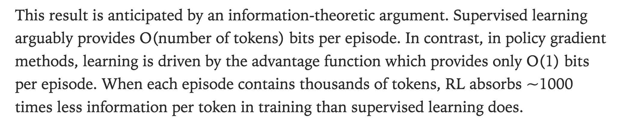 |
| Figure 1: The number of bits provided by SFT vs RL. Extracted from [1]. |
He also gives a concrete back-of-the-envelope: for the MATH dataset, roughly \(10{,}000\) problems × \(32\) samples implies \(\lesssim 320{,}000\) bits if each completion yields ~1 bit. Meanwhile, even rank-1 LoRA on Llama-3.1-8B has \(\sim 3\)M parameters, orders of magnitude more than the training signal, so LoRA should be enough to absord this much information.
The claim sparked a lively debate on Twitter and other adjacent ML spaces. I’ll quote a few representative takes to set the stage:
Prof. Ahmad Beirami on this twitter thread argues:
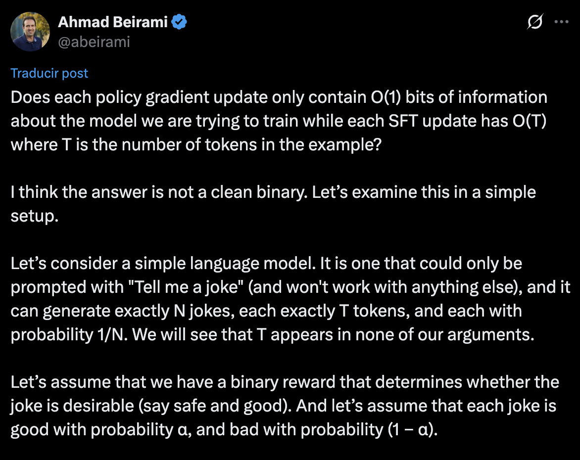 |
| Figure 2: Since the thread is super long i have summarized the main points as: RL with a binary sequence-level reward can reveal at most \(O(1)\) bits per rollout (≤ 1 bit in his toy setup), whereas a positive SFT example can carry \(\log(1/\alpha)\) bits when positives are rare (here \(\alpha\) is the probability a random rollout would succeed). The contrast is not \(O(1)\) vs \(O(T)\) implying that with sequence-level binary rewards, \(T\) doesn’t appear. |
Rishabh Agarwal raises the “surprise” angle here:
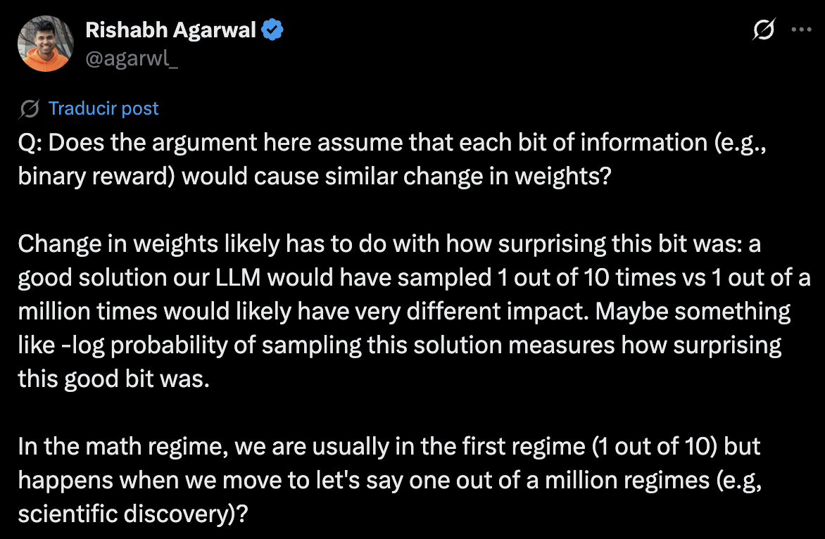 |
| Figure 3: One bit that confirms a very rare good solution (say 1 in a million) should cause a larger weight change than a bit confirming a common solution (1 in 10). How rare a good outcome is matters. |
Susan Zhang emphasizes design choices and that this is not a hard limitation on here:
 |
| Figure 4: The “\(O(1)\) bits per episode” is not fundamental to RL, it’s a property of using only sequence-level binary rewards. If we provide intermediate or token-level rewards, the information per episode can scale with \(T\). |
Dimitris Papailiopoulos and Aryaman Arora discuss gradient dimensionality and have the following exchange here:
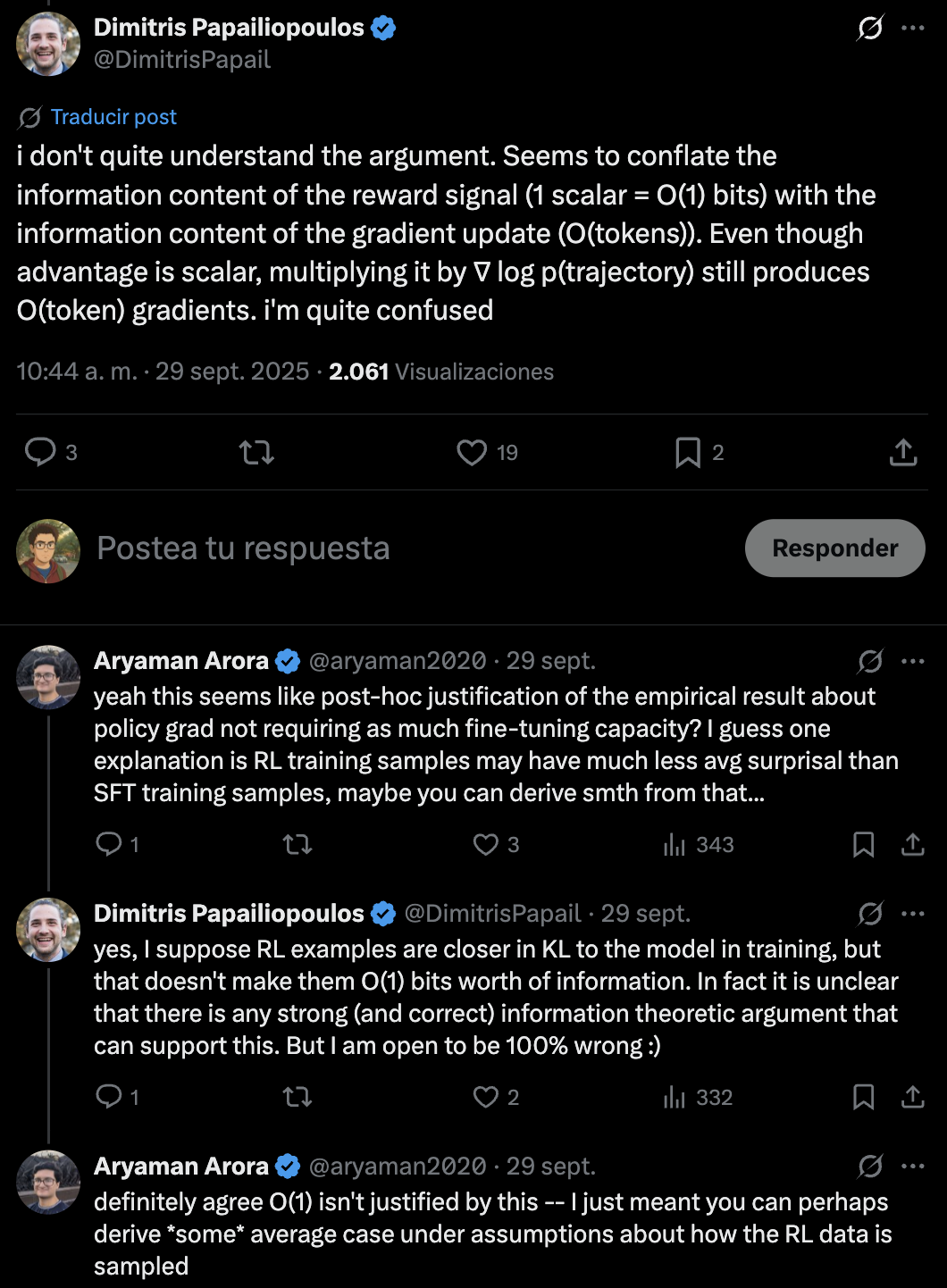 |
| Figure 4: Even if the reward is a single scalar, the gradient is a long vector (roughly \(O(T)\) coordinates). Does that mean the update carries \(O(T)\) information? Or does the scalar bottleneck cap the task-relevant information anyway? |
This posts uses a toy “symbol-emitting bandit” to try to formalize these points and then generalize some of the bounds. The math is simple and uses data-processing and counting arguments. The main takeaways are:
-
Binary sequence-level RL: each rollout update carries ≤ 1 bit; grouped \(K\) rollouts carry at most \(\log_2(K{+}1)\) bits per prompt (often much less because many endings duplicate).
-
SFT positives: a single positive can carry \(\log_2(1/\alpha)\) bits, this value gets larger when successes are rare. If you create positives by filtering rollouts, the per-rollout info returns to \(O(1)\).
-
Dense/token-level rewards: with this per-episode capacity can be \(O(T)\). This is a design choice, not a fundamental limitation of RL (which reinforces Susan’s point).
-
LoRA vs FullFT: If total training signal across RL is \(B\) bits, small adapters can fit it; you don’t need to move all base weights. Moreover, the group-of-\(K\) analysis shows bits grow logarithmically in \(K\), making Schulman’s 1-bit-per-completion conservative in many cases.
I wrote a small scripts to empirically check theese bounds. They’re simple “sanity plots,” not exhaustive experiments. You can find them here
Please note: I am kind of rusty on my information theory, and RL so if you spot mistakes please let me know!!
A simple model: the “symbol-emitting bandit”
Think of a verifiable task (like many math/code problems) where we sample random symbols and the final answer is a single symbol all sampled from a vocabulary \(\mathcal V\).
-
There is a random but verifiable answer: a random variable \(S\in\mathcal V\) .
-
The policy \(\pi_\theta\) samples a trajectory \(\tau=(x_{1:T})\) and emits the last token \(x_T\).
-
Reward: \(r(\tau,S)=\mathbf 1\{x_T=S\}\in\{0,1\}\) (binary, sequence-level).
We make the following on-policy assumption. In a single update step, \(\tau \perp\!\!\!\perp S \mid \theta\): the rollout is drawn from the current policy and is independent of the true answer.
Policy-gradient update (REINFORCE form). For one rollout, an unbiased update looks like
\[\hat g = (r-b)\,\nabla_\theta \log \pi_\theta(\tau),\]
for some baseline \(b\) (possibly computed from a batch). For a group of \(K\) rollouts, \(\hat g\) is a function of \(\{(\tau_i,r_i)\}_{i=1}^K\).
We’ll ask the question: how many bits about \(S\) can \(\hat g\) carry?
The proofs
Binary, sequence-level rewards give at most one bit per rollout
Lemma (One-bit bound).
If \(r=f(S,\tau)\in\{0,1\}\) is binary and \(g=\Phi(\tau,r)\) is any update based on \((\tau,r)\), then
\[I(g;S) \;\le\; I((\tau,r);S) \;=\; I(S;r\mid \tau) \;\le\; H(r\mid \tau) \;\le\; 1.\]
Click to see proof
Data processing gives \(I(g;S)\le I((\tau,r);S)\) because \(g\) is a function of \((\tau,r)\). Since \(\tau\perp\!\!\!\perp S\) we have \(I((\tau,r);S)=I(S;r\mid \tau)\). Finally \(I(S;r\mid\tau)\le H(r\mid\tau)\le 1\) because \(r\) is binary. \(\square\)
For the case of continuous rewards. One would repeat the analysis after a \(b\)-bit quantization \(Q(r)\), yielding \(I(g;S)\le H(Q(r)\mid \tau)\le b\).
Corollary (symbol-bandit). Let the last token be \(T\) and \(r=\mathbf{1}\{T=S\}\) with \(S\) uniform over a vocabulary \(\mathcal V\) of size \(V\). Then
\[I(g;S)\le I((T,r);S)=H(r\mid T)=h(1/V)\le 1,\]
with \(h(\cdot)\) being the binary entropy.
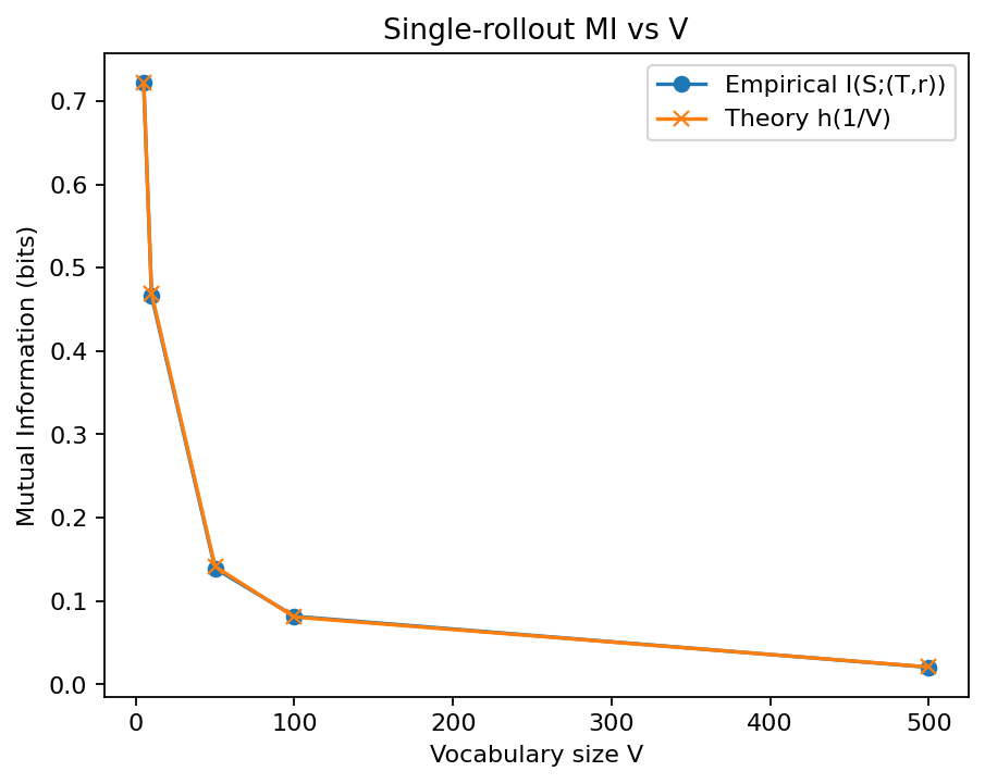 |
| Figure 5: We simulate a uniform policy and measure \(I(S;(T,r))\). Theory says \(I=H(r\!\mid\!T)=h(1/V)\le 1\). We can see that this simple model matches \(h(1/V)\) closely; always \(\le 1\) bit. |
\(K\) rollouts (GRPO/RLOO) and a \(\log(M{+}1)\) bound
For a prompt, draw \(K\) rollouts \((\tau_i)_{i=1}^K\) with binary rewards \(r_i=f(S,\tau_i)\). Let \(M\) be the number of distinct final tokens among the \(\tau_i\). Denote \(\mathbf r=(r_1,\dots,r_K)\).
Theorem (Group bound).
For any update \(g=\Phi(\{\tau_i,r_i\}_{i=1}^K)\),
\[I(g;S) \;\le\; I(\{(\tau_i,r_i)\}_{i=1}^K;S) \;=\; H(\mathbf r \mid \{\tau_i\}) \;\le\; \log_2\!\bigl(M{+}1\bigr),\]
and in particular \(\mathbb E[I(g;S)] \le \mathbb E[\log_2(M{+}1)] \le \log_2(K{+}1)\).
Click to see proof
By data processing, \(I(g;S)\le I(\{(\tau_i,r_i)\};S)\). Using \(\{\tau_i\}\perp\!\!\!\perp S\) and determinism of \(\mathbf r\) given \((S,\{\tau_i\})\), we have
\(I(\{(\tau_i,r_i)\};S)=I(S;\mathbf r\mid\{\tau_i\})=H(\mathbf r\mid\{\tau_i\})\).
Fix \(\{\tau_i\}\). As \(S\) ranges over the vocabulary, \(\mathbf r\) can realize at most \(M\) patterns with ones at positions that share the same final token, plus the all-zero pattern when \(S\) is none of the distinct tokens. Hence at most \(M{+}1\) patterns; entropy is maximized by the uniform distribution, so \(H(\mathbf r\mid\{\tau_i\})\le\log_2(M{+}1)\). Taking expectations and using Jensen yields the stated bounds. \(\square\)
Exact MI under a uniform prior.
If \(S\) is uniform over \(V\) symbols and we only care about the final tokens \(T_i\), then conditionally on \(\{T_i\}\) the distribution of \(\mathbf r\) assigns probability \(1/V\) to each of the \(M\) “one-hot” patterns and \((V{-}M)/V\) to the all-zero pattern, giving
\[I(\{(\tau_i,r_i)\};S)=H(\mathbf r\mid \{T_i\})= \log_2 V - \frac{V-M}{V}\log_2(V - M)\;\le\;\log_2(M{+}1).\]
For this simulation, we sample \(K\) last tokens for each prompt, count \(M\) uniques, and compute the exact MI under uniform \(S\):
\[I = \log_2 V - \frac{V-M}{V}\log_2(V-M).\]
We compare to the average \(\log_2(M{+}1)\) and the loose \(\log_2(K{+}1)\) bound.
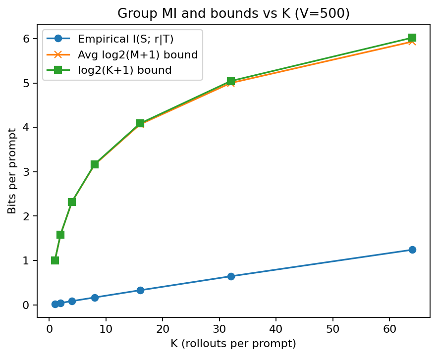 |
| Figure 6: The true MI (given final tokens) is far below \(\log_2(K{+}1)\) when \(V\gg K\). Duplicates keep \(M\) small, so the practical bits per prompt are tiny. |
Let \(\tau^+\) be a positive example consistent with \(S\), drawn so that \(\Pr(\tau^+\text{ occurs})=\alpha\) under the current sampler.
Theorem (Positive-only SFT).
\(I(\tau^+;S)=H(S)-H(S\mid \tau^+)=\log_2(1/\alpha)\) when the example reveals one element of a uniformly distributed good set with prior mass \(\alpha\).
This highlights the ‘cost’ of the SFT example. If an expert gives you a positive example ‘for free,’ you get \(\log_2(1/\alpha)\) bits. If you have to find that positive example by sampling \(\approx 1/\alpha\) rollouts, the total information gained per rollout sampled is still bounded by \(O(1)\), just like in the RL case.
Click to see proof
Let \(\Omega\) be finite with \(|\Omega|=M\). For each solution \(S\), let \(A(S)\subseteq \Omega\) denote the positive set with \(|A(S)|=\alpha M\). By construction, \(\tau^+\mid S \sim \mathrm{Unif}(A(S))\), so
\(
H(\tau^+\mid S) = \mathbb{E}_{S}\big[\log_2 |A(S)|\big] = \log_2(\alpha M).
\)
Assume the \(\alpha\)-symmetry condition that makes the marginal of \(\tau^+\) uniform on \(\Omega\), hence
\(
H(\tau^+) = \log_2 M.
\)
Therefore,
\(
I(\tau^+;S) = H(\tau^+) - H(\tau^+\mid S) = \log_2 M - \log_2(\alpha M) = \log_2(1/\alpha).
\)
\(\square \)
When (and why) you can get \(O(T)\)
Let token-level feedback be \(R_{1:T}=(R_1,\dots,R_T)\) with alphabets \(\mathcal A_t\) (sizes \(A_t\)). The update \(g\) is a function of \((\tau,R_{1:T})\).
Theorem (Token-level capacity).
With \(\tau\perp\!\!\!\perp S\),
\[I(g;S)\;\le\; I((\tau,R_{1:T});S) \;=\; I(S;R_{1:T}\mid \tau) \;\le\; H(R_{1:T}\mid \tau)\;\le\;\sum_{t=1}^T \log_2 A_t.\]
In particular, when each \(R_t\) is binary, \(I(g;S)\le T\) bits.
Click to see proof
Let \(g=\Phi(\tau,R_{1:T})\) with \(R_t\in\mathcal A_t\) (\(|\mathcal A_t|=A_t\)) and assume \(\tau\perp\!\!\!\perp S\).
By data processing,
\(
I(g;S)\le I((\tau,R_{1:T});S)=I(R_{1:T};S\mid\tau).
\)
Then
\(
I(R_{1:T};S\mid\tau)\le H(R_{1:T}\mid\tau) = \sum_{t=1}^T H(R_t\mid R_{1:t-1},\tau) \le \sum_{t=1}^T H(R_t\mid\tau) \le \sum_{t=1}^T \log_2 A_t,
\)
using the chain rule, “conditioning reduces entropy,” and the fact that a discrete variable with at most \(A_t\) outcomes has entropy \(\le \log_2 A_t\).
For binary feedback \(A_t=2\), this gives \(I(g;S)\le T\) bits. \(\square\)
Tightness for binary tokens.
Let each target token \(s_t\in\{0,1\}\) be i.i.d. fair, the policy emits \(x_t\in\{0,1\}\), and define \(R_t=\mathbf 1\{x_t=s_t\}\). Then \(s_t = x_t \oplus (1-R_t)\), so \(S\) is deterministically recoverable from \((\tau,R_{1:T})\) and \(I((\tau,R_{1:T});S)=H(S)=T\) bits. Thus the bound is tight.
We simulate a toy token-level signal \(R_t=\mathbf 1\{x_t=s_t\}\) with fair binary tokens. Theory predicts exactly \(T\) bits.
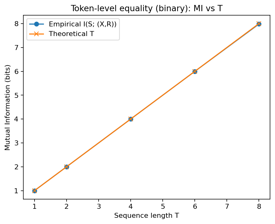 |
| Figure 7: As expected: linear growth in bits with \(T\) when per-token information is present. |
Which RL algorithms use token-level signals? PPO/A2C with per-token advantages, token-level actor-critic/Q-learning, etc. Distributional RL helps with return shapes but is not required for \(O(T)\); the key is giving informative per-step rewards.
Putting it together: what does this mean in practice?
-
In binary, sequence-level RL (many verifiable math setups), the information channel is narrow: ≤ 1 bit per rollout, ≤ \(\log_2(K{+}1)\) bits per grouped prompt. LoRA (even low rank) often suffices to absorb the signal; variance reduction and exploration matter more than raw capacity.
-
In SFT, a positive example can deliver \(\log_2(1/\alpha)\) bits when good outcomes are rare. If your positives are mined from on-policy rollouts, the per-rollout bits are \(O(1)\) again.
-
If you want more bits per episode, change the supervision channel: add token-level checks, intermediate verifications, graded/real rewards, or structured signals (e.g., constraint satisfaction at multiple steps). With such designs, \(O(T)\) bits-per-episode is possible, and algorithm families that consume per-step rewards (per-token PPO/A2C/actor-critic/Q-learning) can use them.
FAQs
“But the gradient is \(O(T)\)-dimensional!”
Yes, but data-processing arguments pin down task-relevant information. Given \(\theta\), the only \(S\)-dependent random variable in a sequence-level binary RL update is the scalar reward (possibly centered). Multiplying a scalar by a long vector does not create new bits about \(S\). Think of the gradient \(\nabla_\theta \log \pi_\theta(\tau)\) as a very long, complex lever. The reward \(r\) is the tiny force (1 bit) you apply to that lever. The lever’s shape determines which of the billions of weights move (the \(O(T)\) dimensionality), but the total amount of task-relevant information driving the push is still just that 1 bit.
“Does GRPO/RLOO add information?”
They reduce variance using group statistics but do not increase the per-prompt bits in the binary case beyond the \(\log_2(M{+}1)\) counting argument. With graded rewards the supervision gets richer and the bound scales accordingly.
“What about exploration and KL?”
Better exploration increases the rate at which useful events happen (wall-clock efficiency) but does not change the per-rollout information bound unless you expand the feedback. KL regularization shapes optimization but doesn’t inject new information about \(S\).
References
[1] Schulman, John and Thinking Machines Lab, “LoRA Without Regret”, Thinking Machines Lab: Connectionism, Sep 2025.
comments powered by